This morning, I’m releasing a live simulation (above) that demonstrates something critical for the future of space operations: Autonomous Causal Learning.
In the simulation, you will see four distinct orbital regimes [including a live digital twin of the ISS] learning the physics of their environment in real-time. You can watch as the system starts with a “Prior” (a best guess based on historical data), encounters an anomaly (like the December 2025 solar storm), and mathematically converges on “Operational Truth.”
While satisfying to watch the cyan bars lock onto reality, it is important to note: This dashboard interface is just for demo purposes.
In our production model, we aren’t tracking four locations. We are tracking 18,000 voxels [3D grid cells that divide orbital space into distinct regions], and enabling action based on those learnings in autonomous devices.
The “Fog of War” in Orbit
There is a dangerous misconception that space is a vacuum of uniform conditions. Currently, most operators rely on global indices like F10.7 (Solar Flux) or Kp (Planetary K-index) to predict atmospheric drag and environmental stress.
Relying on a global index for precise orbital maneuvering is like checking the average temperature of the Northern Hemisphere to decide if you need an umbrella in London. It is simply not granular enough.
As we commercialize space, populating diverse orbits with mega-constellations, building manufacturing hubs, and planning asteroid mining missions, we are hitting the limits of “average” physics.
A 53° Starlink shell experiences different thermospheric heating than a 98° Sun-Synchronous orbit.
Atmospheric density creates drag that varies wildly voxel-by-voxel, capable of dooming a mission or, conversely, offering a free aerobraking maneuver if you know exactly where the density pockets are.
We need a causal model that accounts for these granular conditions to avoid catastrophic losses, optimize thermal strategies for onboard compute, and plan precise navigation paths.
The Nervous Machine: A “Waze for Physics”
This is why we built the Nervous Machine. It operates on a learning architecture of two loops:
1. The Inner Loop (Self-Improving Autonomy) This lives on the edge, on the satellite itself. It uses low-power inference (running on 2-5W) to compare what it expected to happen against what actually happened. When the ISS voxel in the simulation detects that drag is higher than the solar flux should allow, it doesn’t wait for a ground station to tell it what’s wrong. It updates its own causal weights instantly. It closes the Sim-to-Real gap in the last mile.
2. The Outer Loop (Shared Causal Vectors) This is the “Waze” layer. When one car on Waze hits a pothole, every other driver gets alerted. Similarly, when one satellite in our network learns a new physics parameter (e.g., “Auroral heating is 20% higher in Sector 73”), it doesn’t hoard that knowledge.
Crucially, we do not share raw telemetry. Your proprietary data stays on your device. Instead, the system shares Causal Vectors [mathematical representations of the physics].
Satellite A learns: “High drag detected at 480km.”
Satellite B receives: “Update drag coefficient model for 480km.”
The Curiosity Engine: When the Map Doesn’t Match the Territory
The most powerful aspect of the Nervous Machine isn’t how it learns known physics, but how it reacts to the unknown.
In the simulation, you might notice moments where the model has “locked in” [high certainty] on the solar and magnetic conditions, but a residual error persists. The prediction line tracks the observation line, but there is a stubborn gap.
In traditional systems, this is just a bad fit. In our system, this is a Curiosity Trigger.
The logic is simple but profound:
“If I am 90% certain about the Solar Wind impact, and 95% certain about the Auroral heating, but I am still seeing 20% more drag than predicted... then there must be a missing edge in my causal graph.”
Example: The Debris Strike
Imagine a satellite in a 53° shell experiences a sudden, unpredicted drag spike.
Check Knowns: The model checks its internal priors. Is there a solar storm? No. Is the attitude thruster firing? No. The known causal weights are stable (Z > 0.8).
Trigger Curiosity: Because the knowns are stable but the error is high, the system flags a “Causal Dissonance.”
Hypothesize & Validate: The edge device escalates the anomaly. It doesn’t just send an error code; it asks a question.
Is this a sensor malfunction?
Is this a localized density bloom?
Is this a debris interaction?
This allows the system to autonomously trigger a literature search, query an LLM for similar anomalies in that orbital regime, or alert a human operator with a specific hypothesis rather than a generic alarm. It transforms the satellite from a passive data collector into an active investigator.
Why This Matters Now
This architecture doesn’t just drive self-improvement in a single device, it enables Fleet Learning. If one satellite encounters an anomaly, the entire fleet, and eventually the entire orbital economy, becomes smarter and safer.
We are moving past the era of “guess and check” in orbit. By deploying 18,000 voxel-level models, we turn space from a chaotic, unknown environment into a mapped, navigable domain.
Play with the simulation: http://nervousmachine.com/voxels. Watch the system learn. Then imagine that capability scaled across the entire sky.
Under the Hood: The Math of Certainty
If you are watching the simulation and wondering why the “Learned Weight” bars move quickly at first and then stabilize, you are seeing Dissipative Learning in action.
In a standard neural network, the learning rate is usually fixed or decays on a schedule. In the Nervous Machine, the learning rate η is a function of the voxel’s own Causal Certainty (Z).
We use a sigmoidal decay function to modulate plasticity:
Where:
Z (Certainty) is the confidence the voxel has in its current physics model (0.0 to 1.0).
α is the base plasticity (how fast can we learn?).
k is the “lock-in” factor (how hard is it to change our mind?).
Why this matters:
Low Certainty (Z < 0.2): The system is “agile.” It admits high error signals to rapidly approximate the environment. (This is why the bars jump when you start).
High Certainty (Z > 0.8): The system becomes “stubborn.” It resists noise and outliers. It requires a sustained, coherent error signal (like a persistent atmospheric density change) to overwrite its prior knowledge.
This is how we prevent Catastrophic Forgetting on the edge. A single debris strike (a noisy outlier) won’t retrain the model, but a genuine shift in the thermosphere will.
The Curiosity Threshold: We mathematically define curiosity as the state where Certainty (Z) is high, but Error (ε) remains above a tolerance threshold (Z > 0.85 ∧ ε > 0.15). This is the mathematical signal that triggers hypothesis generation.


